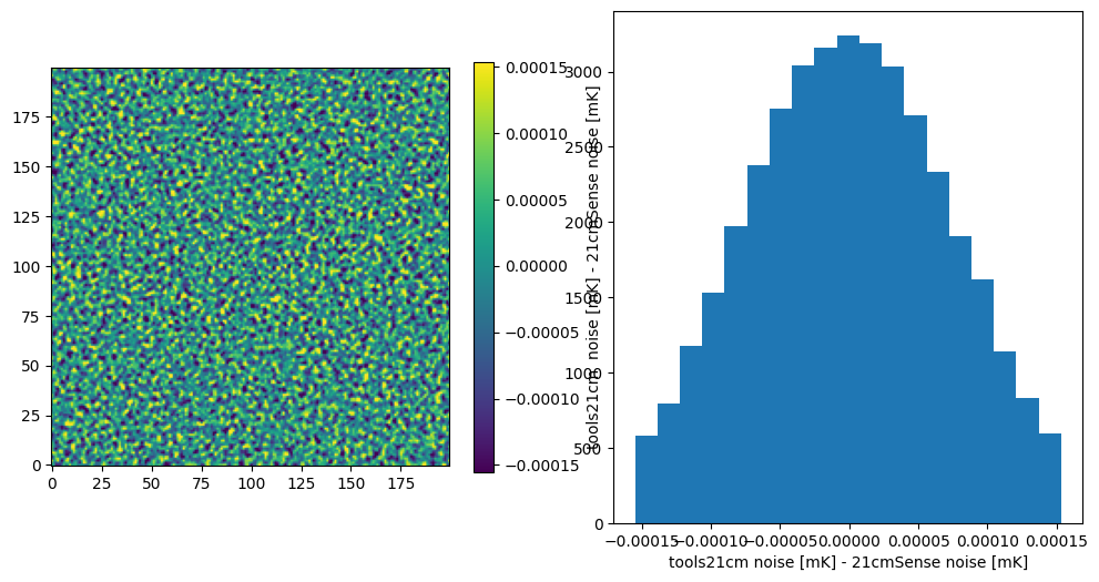
Generating lightcone noise samples - Comparing between tuesday and tools21cm
tools21cm (master branch on 01/07/25, commit c0cc4d5) with tuesday. We do this using the AA4 SKA layout.[1]:
import numpy as np
from py21cmsense import Observatory, Observation
from py21cmsense.conversions import f2z
import astropy.units as un

from tools21cm.radio_telescope_noise import get_uv_map, get_SKA_Low_layout
import matplotlib.pyplot as plt
[2]:
def compare(tools_qt, tuesday_qt, qt_name="", f = "150 MHz", vmin=None, vmax=None):
    fig, axs = plt.subplots(1, 3, figsize=(12, 6), gridspec_kw={"width_ratios":[1,1,0.07]})
    if vmin is None:
        vmin = np.nanpercentile(tools_qt, 2.5)
    if vmax is None:
        vmax = np.nanpercentile(tools_qt, 97.5)
    axs[0].set_title(f"tuesday - {qt_name} at {f} for SKA AA4")
    axs[0].imshow(np.flip(tuesday_qt.T), origin="lower", vmin = vmin, vmax = vmax)
    axs[1].set_title(f"tools21cm - {qt_name} at {f} for SKA AA4")
    im=axs[1].imshow(tools_qt.T, origin="lower", vmin = vmin, vmax = vmax)
    fig.colorbar(im,  label = qt_name, cax = axs[2],fraction=0.1,shrink=0.6)
    plt.show()
    err = tools_qt.T - np.flip(tuesday_qt.T)
    vmin = np.nanpercentile(err, 2.5)
    vmax = np.nanpercentile(err, 97.5)
    fig, axs = plt.subplots(1,2, figsize=(12, 6))
    im = axs[0].imshow(err, vmin = vmin, vmax = vmax, origin="lower")
    fig.colorbar(im,  label = f"tools21cm  {qt_name} - 21cmSense {qt_name}", fraction=0.1,shrink=0.8)
    axs[1].hist(err.ravel(), bins = np.linspace(vmin,vmax,20))
    axs[1].set_xlabel(f"tools21cm {qt_name} - 21cmSense {qt_name}")
    plt.show()
Compare SKA AA4 layouts
We check that the station layouts used in both codes are the same:
[3]:
hours_tracking = 6.*un.hour
observatory = Observatory.from_ska("AA4")
freqs = np.array([150.0, 250.0]) * un.MHz
[4]:
enu_coords = get_SKA_Low_layout("AA4", unit="enu")
AA4 contains 512 antennae.
[5]:
plt.scatter(enu_coords[:,0], enu_coords[:,1], color = "k", label = "tools21cm")
plt.scatter(observatory.antpos[:,0], observatory.antpos[:,1], color = "r", marker = ".", label = "tuesday")
plt.legend()
plt.show()
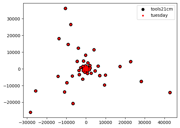
tools21cm and 21cmSense are using the same SKA antenna layout.tuesday With tuesday, the user can use the Observatory object along with the integration time and daily observation duration to calculate the location of a reference point through zenith as the sky rotates overhead during the day. This will provide us with daily observation duration in s / integration time in s time offsets.[6]:
observatory = observatory.clone(beam=observatory.beam.clone(frequency=freqs[0]))
integration_time = 60*un.s
time_offsets = observatory.time_offsets_from_obs_int_time(integration_time, hours_tracking)
Once we have the time offsets, the last missing ingredient is to obtain the baseline groups of the instrument and the weights of each (i.e. how many baselines are in a given group):
[7]:
baseline_groups = observatory.get_redundant_baselines()
baselines = observatory.baseline_coords_from_groups(baseline_groups)
print("We have", baselines.shape[0], "baseline groups.")
weights = observatory.baseline_weights_from_groups(baseline_groups)
bl_max = np.sqrt(np.max(np.sum(baselines**2, axis=1)))
finding redundancies: 100%|██████████| 511/511 [00:01<00:00, 468.57ants/s]
We have 261582 baseline groups.
[8]:
from tuesday.core import grid_baselines_uv
Now that we have the baseline groups and the time offsets, we take the baseline groups and move them for each time offset as the sky rotates over the instrument:
[9]:
proj_bls = observatory.projected_baselines(baselines=baselines, #21cmsense caches them
                                           time_offset = time_offsets, ) #(Nbls, N time_offsets, 3)
[10]:
lc_shape = np.array([200,200,1945])
boxlength = 300. *un.Mpc
We can grid the baselines now. Note that in this step we decimate the baseline and their weight arrays by two. This is because these array originally contain both the positive baselines \(\textit{and}\) their mirrored copy i.e. (u,v) and (-u,-v) which do not contribute to reducing our SNR (since they’re the same). The grid_baselines_uv assumes we provide only one copy of the baselines and is a little bit faster that way. We loop over the frequencies and rescale the baselines accordingly.
[11]:
uv_coverage = np.zeros((lc_shape[0],lc_shape[0],len(freqs)))#Nu, Nv, Nfreqs
for i, freq in enumerate(freqs):
    # uv coverage integrated over one field
    uv_coverage[...,i] += grid_baselines_uv(proj_bls[::2]*freq/freqs[0],
                              freq,
                        boxlength,
                        lc_shape,
                        weights[::2])
Calculate uv coverage with tools21cm
[12]:
redshifts = [f2z(freq) for freq in freqs]
uv_tools = np.zeros_like(uv_coverage)
for i,z in enumerate(redshifts):
    uv, Nant = get_uv_map(lc_shape[0],z,
                                 boxsize=boxlength.value,
                                 int_time=integration_time.value,
                                 total_int_time= hours_tracking.value,
                                 include_mirror_baselines=True,
                                 declination = -26.824722)
    uv_tools[...,i] = np.fft.fftshift(uv)*int(3600*hours_tracking.value/integration_time.value)
AA4 contains 512 antennae.
ENU -> ECEF -> XYZ
Generating uv map from daily observations...
Gridding uv tracks: 100%|██████████| 360/360 [00:05<00:00, 65.89it/s]
...done
AA4 contains 512 antennae.
ENU -> ECEF -> XYZ
Generating uv map from daily observations...
Gridding uv tracks: 100%|██████████| 360/360 [00:05<00:00, 70.28it/s]
...done
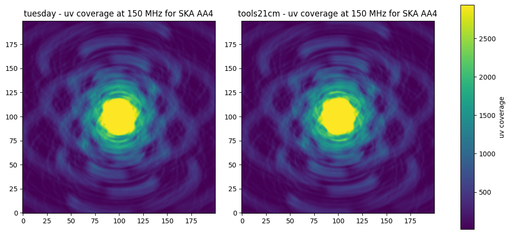
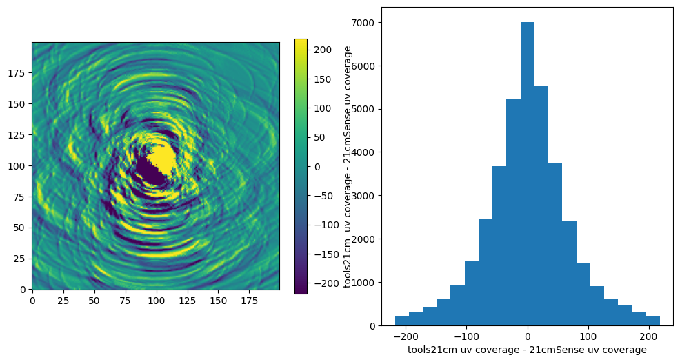
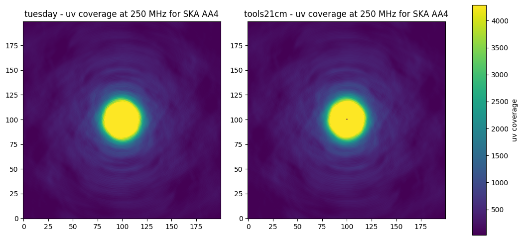
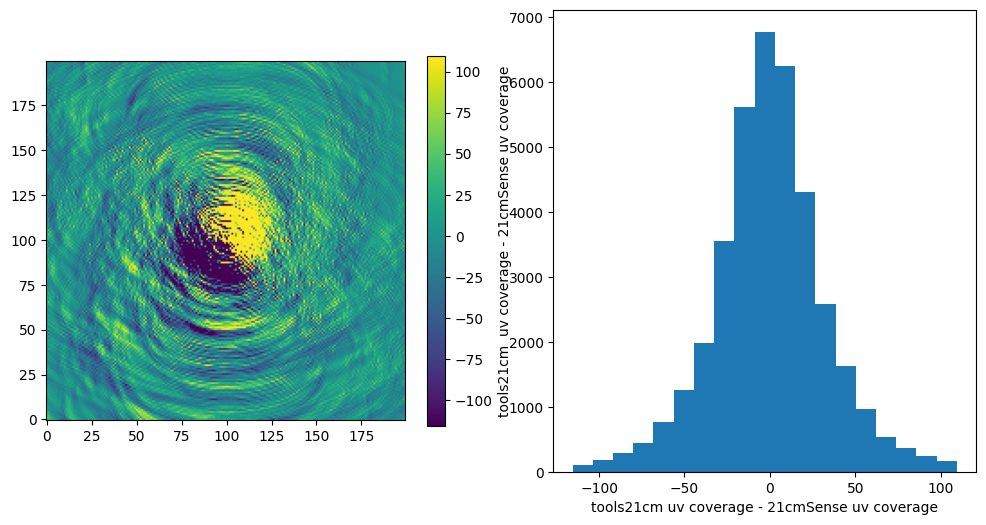
Compare uv coverage
[13]:
compare(uv_tools[...,0], uv_coverage[...,0], "uv coverage", f = "150 MHz")
[14]:
compare(uv_tools[...,1], uv_coverage[...,1], "uv coverage", f = "250 MHz")
Calculate the thermal RMS noise with tuesday
To calculate the thermal noise with tuesday, we need to define an Observation. Note that we choose \(T_{\rm sky}\) parameters to match those in tools21cm.
[15]:
from tuesday.core import thermal_noise_per_voxel
[16]:
# Define an observation
obs = Observation(observatory=observatory.clone(beam=observatory.beam.clone(frequency=freqs[0])),
            time_per_day=hours_tracking,
            lst_bin_size=hours_tracking,
            integration_time=integration_time,
            bandwidth=50 *un.kHz,
            n_days=int(np.ceil(1000/hours_tracking.value)),
            tsky_amplitude=60.*un.K,      # to be consistent with tools21cm
            tsky_ref_freq=300.*un.MHz,
            spectral_index=2.55,
                 )
[17]:
sigmaN_rms = thermal_noise_per_voxel(obs, freqs, boxlength, lc_shape, antenna_effective_area = [517.7, 186.4]*un.m**2) #A_eff set to match tools21cm
sigmaN = sigmaN_rms / np.sqrt(uv_coverage * obs.n_days)
sigmaN[uv_coverage == 0.] = 0.
Calculate thermal RMS noise with tools21cm
[18]:
from tools21cm.radio_telescope_sensitivity import sigma_noise_radio, jansky_2_kelvin, kelvin_2_jansky
from tools21cm.radio_telescope_noise import noise_map
[19]:
sigmaN_tools = np.zeros((lc_shape[0],lc_shape[0],len(freqs)))#Nu, Nv, Nfreqs
sigmaN_rms_tools = np.zeros(len(freqs))

for i, freq in enumerate(freqs):
    sigma, rms_noi = sigma_noise_radio(f2z(freq),
                                       obs.bandwidth.to(un.MHz).value,
                                       obs.n_days*obs.time_per_day.value,
                                       integration_time.value,
                                       uv_map=uv_tools,
                                       N_ant=512) #μJy
    sigmaN_rms_tools[i] = jansky_2_kelvin(rms_noi*1e-6, f2z(freq), boxsize=boxlength.value, ncells=lc_shape[0])[0] #mK
    print("RMS tools21cm",sigmaN_rms_tools[i], "vs RMS tuesday", sigmaN_rms[i])
    sigmaN_tools[...,i] = sigmaN_rms_tools[i] / np.sqrt(uv_tools[...,i] * obs.n_days)
sigmaN_tools[uv_tools == 0.] = 0.
Expected: rms in image in µJy per beam for full = [11.08944821]
Effective baseline = [0.5803084] m
Calculated: rms in the visibility = [983444.49945772] µJy
RMS tools21cm 56.17219074438801 vs RMS tuesday 54.23851346114949 mK

Expected: rms in image in µJy per beam for full = [13.33978878]
Effective baseline = [0.69806823] m
Calculated: rms in the visibility = [1183011.2419225] µJy
RMS tools21cm 16.964242498442857 vs RMS tuesday 16.51463278087388 mK
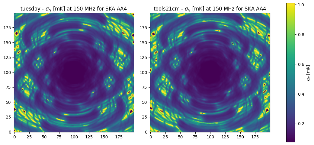
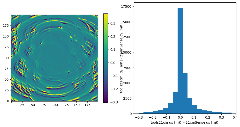
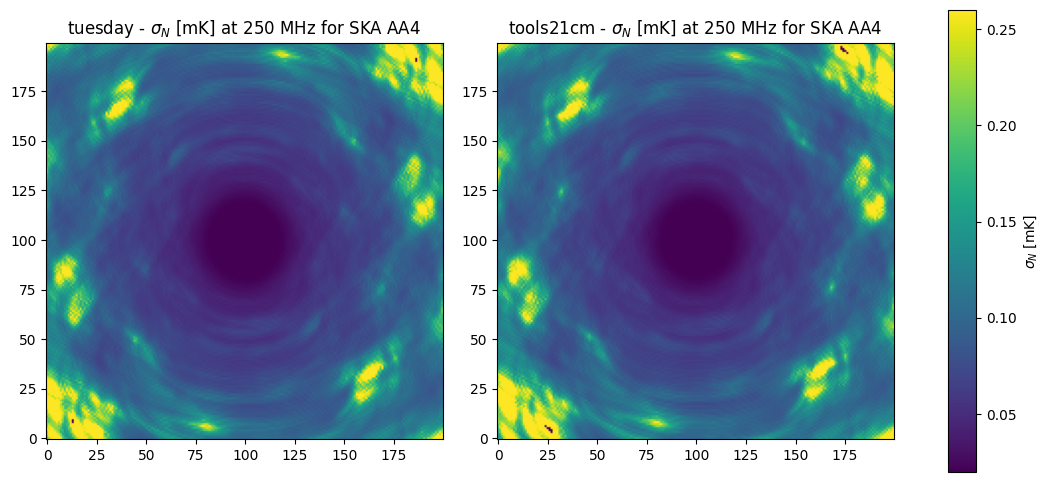
Compare the thermal RMS noise
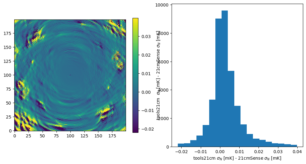
[20]:
compare(sigmaN_tools[...,0], sigmaN[...,0].value, r"$\sigma_{N}$ [mK]")
[21]:
compare(sigmaN_tools[...,1], sigmaN[...,1].value, r"$\sigma_{N}$ [mK]", f="250 MHz")
Sample lightcone noise with tools21cm
The final step is to generate lightcone noise samples.
[22]:
from tools21cm.radio_telescope_noise import noise_map
[23]:
noise_tools = np.zeros_like(sigmaN)
for i, freq in enumerate(freqs):
    n = noise_map(lc_shape[0],
                        f2z(freq),
                        obs.bandwidth.to(un.MHz).value,
                        obs_time=obs.n_days*obs.time_per_day.value,
                        subarray_type="AA4",
                        boxsize=boxlength.value,
                        total_int_time=obs.time_per_day.value,
                        int_time=integration_time.value,
                        declination=-26.824722,)*un.uJy
    noise_tools[...,i] = jansky_2_kelvin(n.to(un.Jy).value, f2z(freq), boxsize=boxlength.value, ncells=lc_shape[0])*un.mK
AA4 contains 512 antennae.
ENU -> ECEF -> XYZ
Generating uv map from daily observations...
Gridding uv tracks: 100%|██████████| 360/360 [00:05<00:00, 65.22it/s]
...done
AA4 contains 512 antennae.
ENU -> ECEF -> XYZ
Generating uv map from daily observations...
Gridding uv tracks: 100%|██████████| 360/360 [00:05<00:00, 70.00it/s]
...done
Sample lightcone noise with tuesday
tuesday we can control the random generation by setting a random seed manually for reproducibility. If not set, a seed is chosen at random.nsamples.[24]:
from tuesday.core import sample_lc_noise
[25]:
noise = sample_lc_noise(sigmaN,
                        seed=4,
                        nsamples=10)
Compare noise realisations
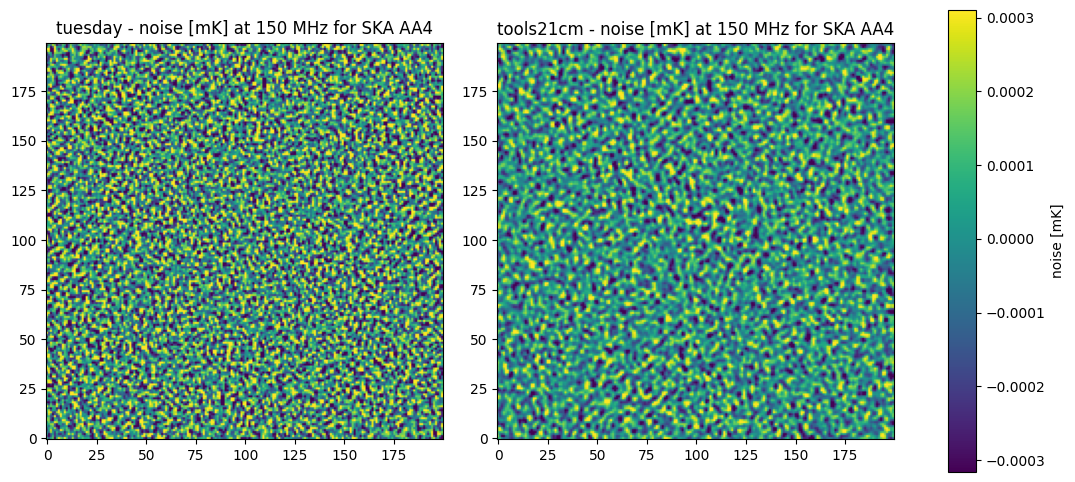
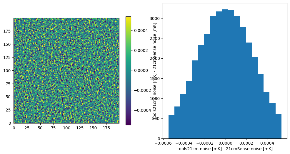
[26]:
compare(noise_tools.value[...,0], noise[2,...,0].value, "noise [mK]")
[27]:
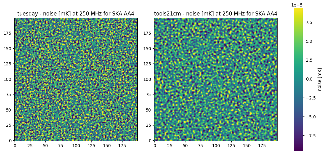
compare(noise_tools.value[...,1], noise[0,...,1].value, "noise [mK]", f="250 MHz")
[ ]: